In the article about blending modes I also described some blending modes or showed the results of blending modes that are not part of Substance 3D Designer. Perhaps some of you have wondered how I did this. The answer is: “With the Pixel Processor!” (Any other answer would probably have been confusing given the title of this article 😉) And in this article, I would like to show you exactly how I did it.
What is the Pixel Processor?
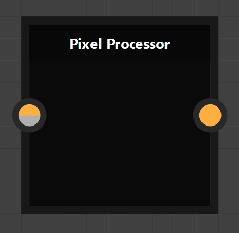
New Pixel Processor
Alongside FxMap, the pixel processor is one of the most powerful nodes in Substance 3D Designer, even if it seems rather useless at first. This is because the pixel processor does nothing at all on its own and only delivers a black image as a result, regardless of the input. The power of the pixel processor is revealed when you edit the “Per Pixel Function” and fill it with life. To do this, either click on the “Edit function” below “Per Pixel Function”, which can be found under the “Specific Parameters” of the pixel processor, or simply press Ctrl + E.

Empty function graph
You are then greeted with a new empty graph. If you look at the available nodes, you will undoubtedly have to think about math lessons for a moment if you have no experience with shaders. But for now, it’s all half as bad. As the name of the parameter suggests, this graph or function is called for each individual pixel of the input image, i.e. a good 1 million times for a 1024x1024 image, and is therefore somewhat comparable to a fragment/pixel shader.
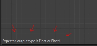
Expected output value (lower left corner of the function graph)
The bottom left of the window shows what the graph expects as output. In the case of the pixel processor, it is either a Float or a Float4, i.e. either a grayscale or an RGBA value.
Simple examples
I have come up with a few simple examples to get you started. They have been chosen in such a way that we can increase the complexity of each example without having to worry about complex formulas.
Probably the simplest Pixel Processor
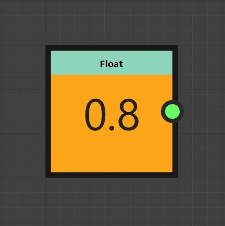
Simplest Pixel Processor
Probably the easiest way to fill the “Per Pixel Function” with life is to create a static output by coloring each pixel light grey, for example. To do this, we create a “Float” node, give it the value \(0.8\) and declare this node as the output node by selecting “Set as Output Node” in the context menu of the node (right-click). If this works, the background color of the node changes to orange. Thus, for each call, i.e. pixel, we return the value \(0.8\), which in Substance 3D Designer (value range 0 - 1) represents a light gray for grayscale.

Result of the simplest Pixel Processor
The first own linear gradient
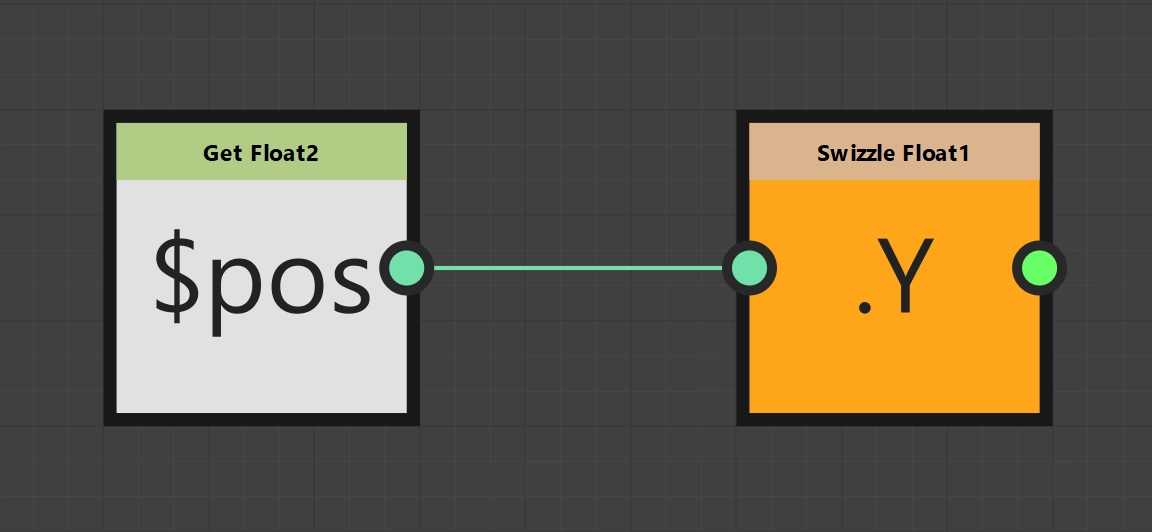
Generation of a vertical gradient in the pixel processor
Now that we know how to assign the same value to each pixel, let’s make it a little more flexible and create a linear gradient. We now need to know which pixel we are creating. There is a Float2 variable called $pos, which we can read out with the help of the Get Float2 node by selecting the variable directly in the drop-down field or writing it in ourselves. The X and Y values of the position also range from 0 to 1, with pixel (0, 0) always denoting the top left corner and pixel (1, 1) the bottom right corner. For a horizontal gradient we therefore need our X position and for the vertical version our Y position. To split a vector, there are various “swizzle” nodes, depending on how many values you want to have at the end. We only want to have one value, so we take the Swizzle Float 1 node and select either X or Y depending on the desired result. We then declare the Swizzle Float 1 node to be our output node again and we have a linear gradient 🎉

Generated vertical gradient
Looping through an input image
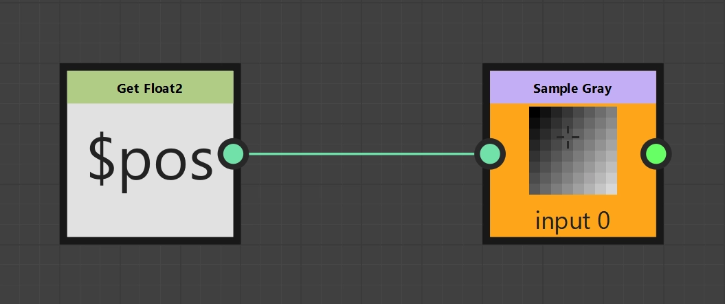
Looping through an input image
Finally, we need to look at how we access input images. The current pixel position $pos is essential here too, of course, but we also need a Sample node. There are two types of Sample nodes, Sample Color and Sample Gray, which provide either RGBA or grayscale values according to their names. They each expect a Float2 as input, i.e. the desired pixel position. To simply output an image unchanged, i.e. to loop it through, we connect our current pixel position to the Sample node of our choice and declare the Sample node to be the output node. This completes the looping of an input image.
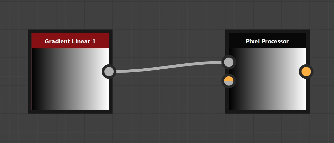
Pixel Processor in application
Replication of blending modes
Now that we understand the basics, let’s focus on tasks that are easy to check. We will recreate blending modes already integrated in Substance 3D Designer and can check ourselves by comparing our result with the integrated version.
Add
Let’s start again with a simple blending mode: Add.
As a reminder, the formula was: \(p_\text{new} = p_\text{bg} + p_\text{fg}\)
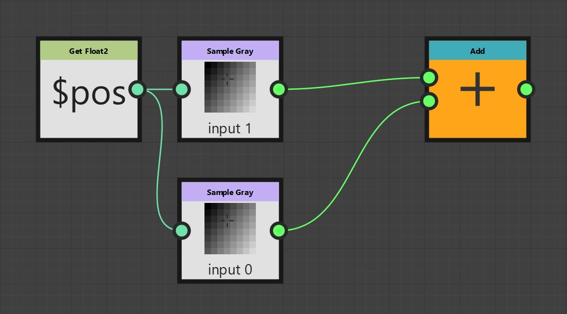
Add function
We create a new pixel processor and supply it with the desired input data. We use the integrated blend node as a guide, so that the upper input will be the foreground image and the input below will be the background image.
We access the current pixels via Sample nodes. In the options of the Sample nodes, you can configure which input image is to be used. The first image (top input) is “Input Image 0”, the second image correspondingly “Input Image 1”. As usual, we use our current pixel position $pos as the input value for both Sample nodes. The last step is to add both values, which is done with the “Add” node, which is then also declared as the output node.
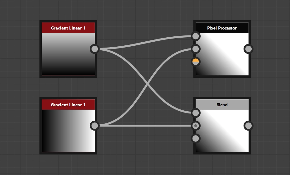
Pixel Processor in application incl. comparison with the original solution
Soft Light
Let’s increase the level of difficulty a little by recreating a more complex blending mode: Soft Light.
As a reminder, the formula of the integrated version was:
\( p_\text{new} = \begin{cases} 2 p_\text{bg} p_\text{fg} + p_\text{bg}^2 (1 - 2 p_\text{fg}) & p_\text{fg} \lt 0.5 \\ \sqrt{p_\text{bg}} (2 p_\text{fg} - 1) + 2 p_\text{bg} (1 - p_\text{fg}) & \, \text{otherwise} \end{cases} \)
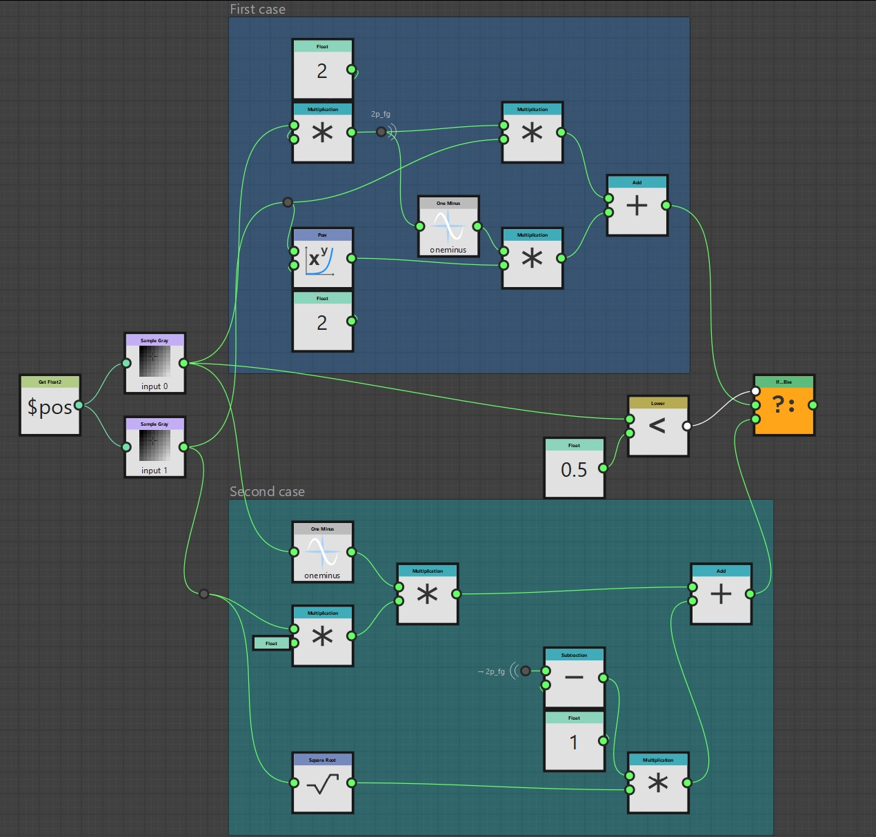
Soft Light function
The formula may be very complex compared to the previous examples, but if we simply reproduce it step by step, it is not much more difficult than in the previous examples, just longer 😉
The basic graph looks the same as in our add. We need our current pixel position $pos and two Sample nodes, i.e. one for each input image.
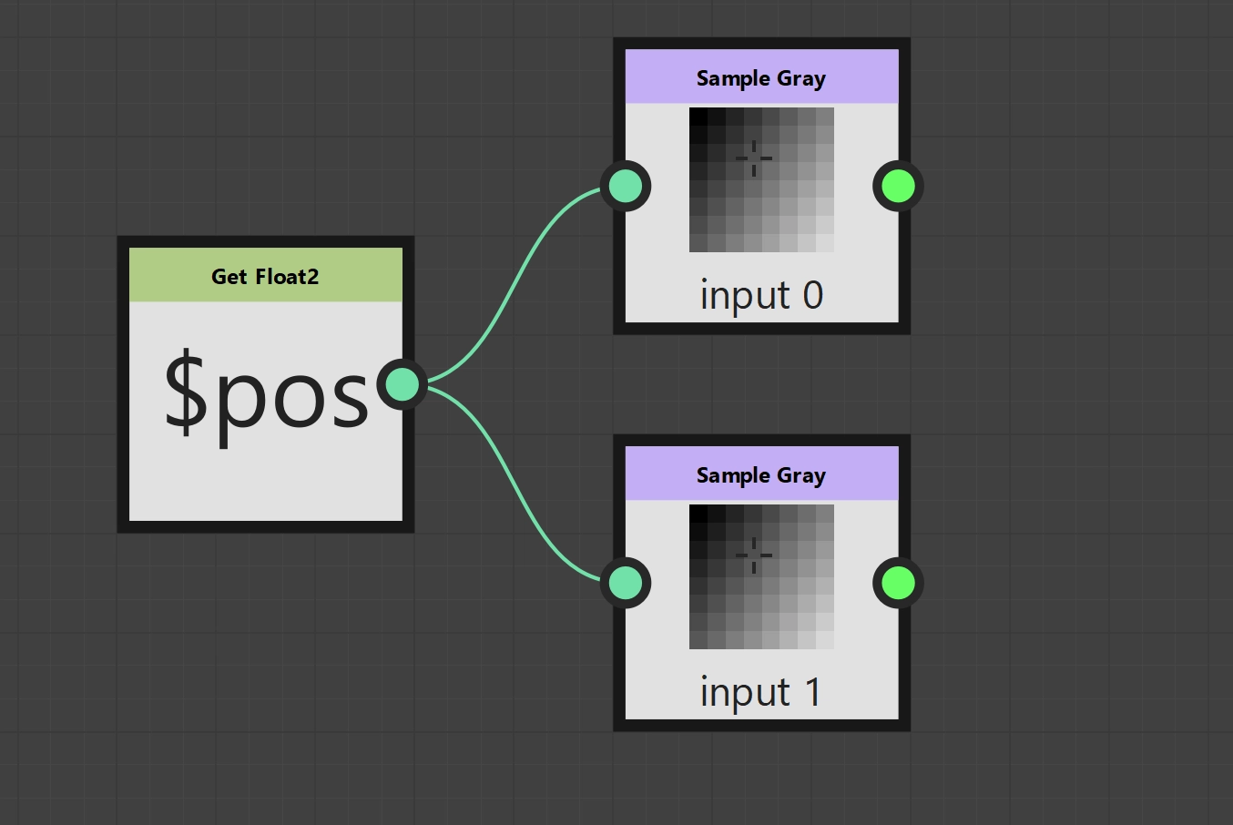
Soft Light function (basic layout)
Let’s start with the first subterm: \(2 * p_\text{bg} * p_\text{fg}\). We therefore need a Float node with the value 2 and two Multiply nodes, which we connect to our Sample nodes.
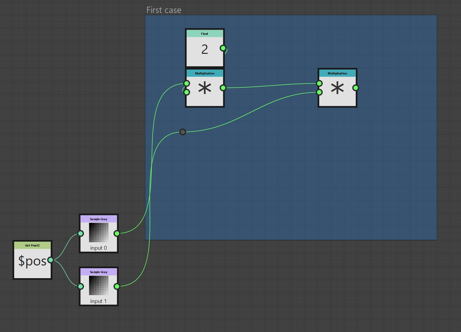
Soft Light function (1. subterm)
The second subterm is \(p_\text{bg}^2 (1 - 2 p_\text{fg})\). If you paid close attention to the previous subterm, you will notice that I have changed the order of the multiplications. So we can also use an intermediate result for this subterm. The Pow node exists for squaring and a One Minus node exists for the subtraction of 1, so that we now only have to connect everything appropriately. We then add our two partial terms so that we have already replicated the first case.
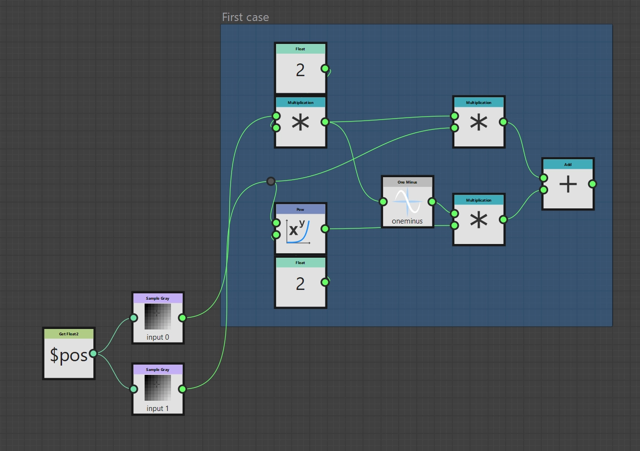
Soft Light function (1. Case)
In the second case, we also proceed step by step and divide the entire term into the two summands. So we start with \(\sqrt{p_\text{bg}} (2 p_\text{fg} - 1)\). We can take the square root using the Square Root node. Subtraction is of course possible with the Subtraction node. Here, too, we can reuse our intermediate result \(2 * p_\text{fg}\) from the first subterm.
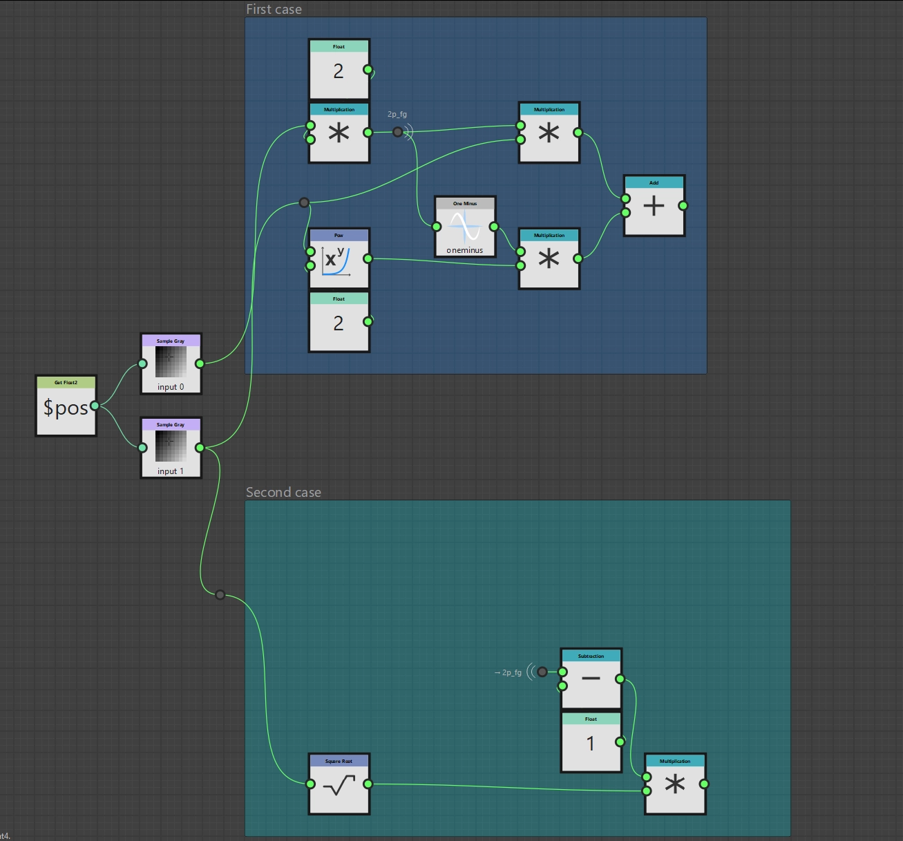
Soft Light function (2. Case, 1. Subterm)
Now we come to the last subterm \(2 * p_\text{bg} * (1 - p_\text{fg})\). We have already learned all the required nodes, so the result should come as no surprise.
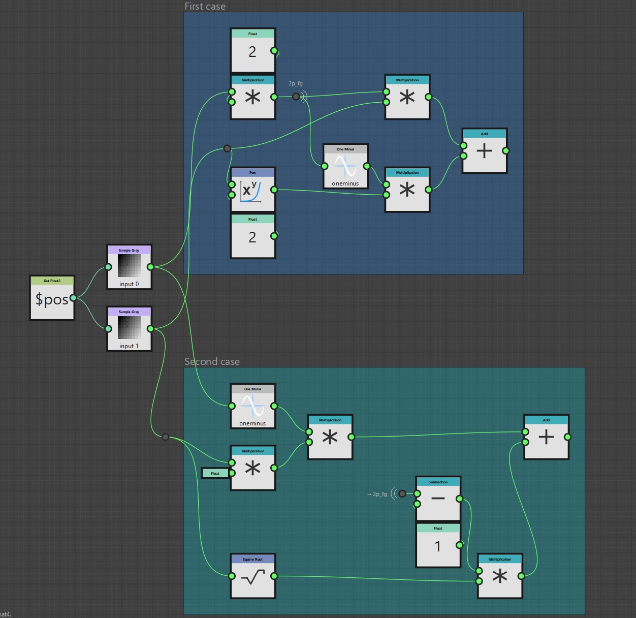
Soft Light function (2. Case)
Last but not least, we now have to implement the case differentiation. Of course, there is also a suitable node for this, the If...Else node. The If...Else node has the three inputs Condition, If and Else. If Condition applies, the input of If is passed on, otherwise that of Else. For the comparison we still need the Lower node and then it’s time to wire it up. Finally, we declare the If...Else node to be the output node and our own implementation of Soft Light is ready.

Soft Light function
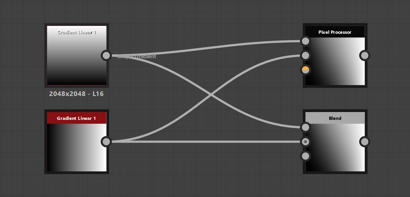
Pixel Processor in application incl. comparison with the original solution
Creating own functions
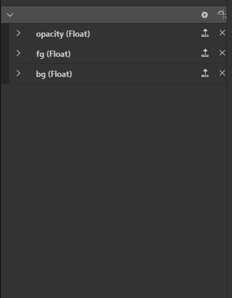
Input parameters Opacity function
In the last part of this article, I would now like to integrate the opacity. As we know from my last article, opacity is independent of the blending mode. We can therefore take the trouble to implement it once so that we can then use it in every blending mode. So that we don’t always have to do this by copy’n’paste, we use a function for this. We create the function by creating a new “Substance function graph” in our current “Substance Package” and appropriately naming it “Opacity”.
For the implementation, we use the familiar formula from the last article: \(p_\text{opa} = O * p_\text{new} + (1 - O) * p_\text{bg}\)
So we have three input values that we have to combine, all of which are Float values. In order to have access to input values at all, we have to declare them in our function, which, as usual with Substance 3D Designer, is done within the “Parameters”. We therefore create three Float values and name them opacity, fg and bg.
As all input values are Float values, we can use the Get Float node three times. We must now select or enter the name of the appropriate input parameter as the name of the value to be read. All other operations should also be known, so we can quickly create two Multiplication nodes, a One Minus node and an Add node and then wire up the formula. Finally, we declare our Add node to be the output node and the programming of the function is complete.
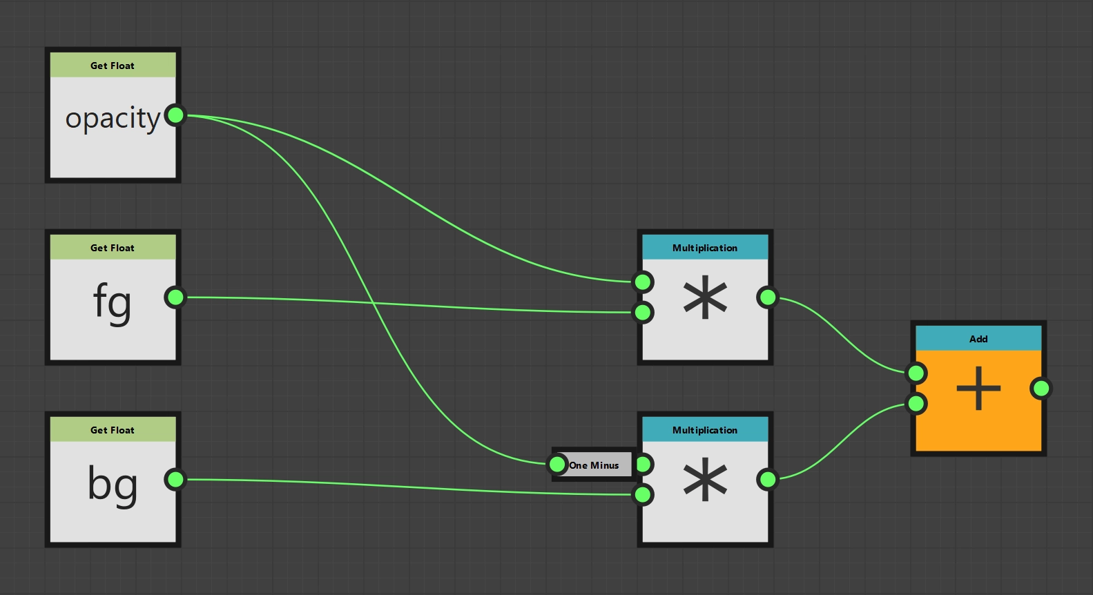
Opacity function
Finally, we can now integrate our function into our already implemented blending modes. The first step is to give our Pixel Processor node a new input parameter #opacity. In the next step, we go to the respective Per Pixel Function and drag in our freshly programmed Opacity function. This gives us a node with three input parameters and one output parameter, which is now declared as our new output node. In order for it to perform its task, we just have to integrate it correctly. As fg we use the previous output node, as bg the sample node of the input background and for opacity we still have to read out our newly created parameter and pass it on. All in all, the function graphs should look something like this.
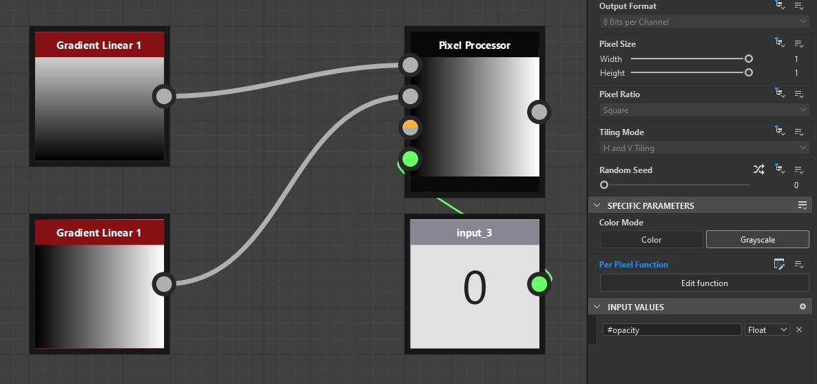
Setup for using the Opacity function
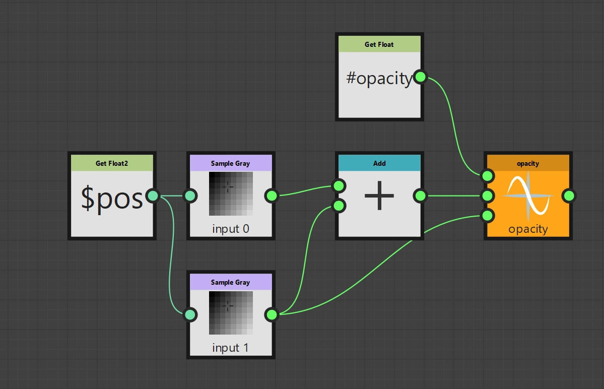
Add mode with Opacity function
Bottom line
I hope this introduction was at least as interesting and exciting for you as the conception and creation of the article was for me. I hope that I have been able to give you a good first impression of the potential power of the pixel processor, because what I have shown here so far have only been simple examples. With the basics, it is now possible for you to implement any pixel-based algorithm and create nodes that do exactly what you want them to do.
